"암호화폐 채굴에 데이터센터·반도체 팹까지" 전력난에 신음하는 美 텍사스, 경고 쏟아져 나와
"암호화폐 채굴에 데이터센터·반도체 팹까지" 전력난에 신음하는 美 텍사스, 경고 쏟아져 나와

입력
수정
美 텍사스주, 산업 구조 전환 속 전력 수요 폭증
암호화폐 채굴 업체·AI 데이터센터가 전력망 부하 키워
줄줄이 들어서는 반도체 공장도 부담 요인으로 지목
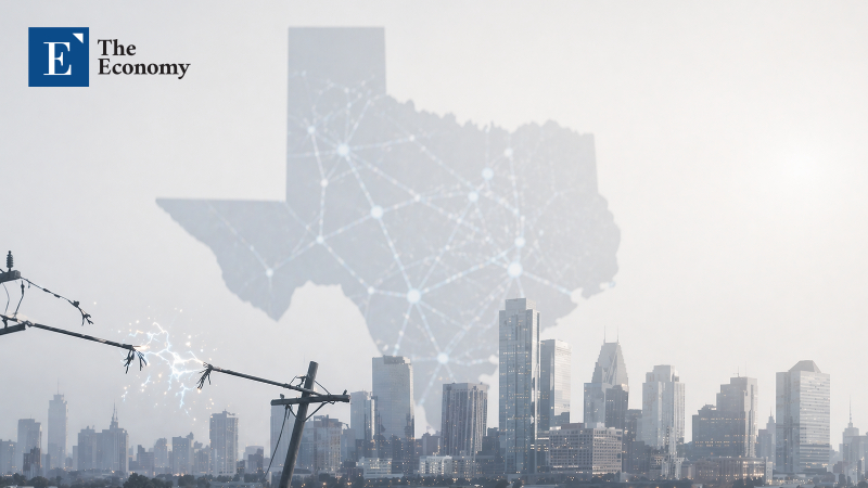
미국 텍사스주의 전력 수요가 급속도로 증가하고 있다. 대규모 암호화폐 채굴 클러스터가 이미 막대한 전력을 소모하는 가운데, 인공지능(AI) 데이터센터 건립 수요까지 속속 텍사스로 몰리며 전력망 부하가 가중되는 양상이다. 이에 더해 텍사스에 자리 잡은 삼성전자, 테슬라 등의 반도체 생산 거점들 역시 관련 리스크를 키우는 요인으로 꼽힌다.
텍사스 전력망 '비상'
23일(현지시각) 미국 경제 매체 제로헤지의 보도에 따르면, 최근 텍사스전기신뢰성위원회(ERCOT)는 오는 2030년대 초반 텍사스 내 전력 피크 수요가 36만7,790메가와트(MW)에 달할 수 있다는 전망을 제시했다. 이는 텍사스주가 지난 2023년 8월에 기록한 역대 최대 피크 수요(8만5,508MW)의 4.3배에 달하는 규모다. ERCOT는 텍사스 전력망을 운영하는 독립 계통 운영기관(ISO)이자, 텍사스 전력 수요의 약 90%를 담당하는 단일 전력망 운영 주체다.
앞서 ERCOT는 지난해 발간한 '전력 용량, 수요 및 보유' 보고서에서도 전력 위기를 경고한 바 있다. 오는 2027년 텍사스에서 최대 8.3%의 전력 공급 부족이 발생할 가능성이 있으며, 2029년 여름에는 부족 비율이 32.4%로 뛸 수 있다는 분석이다. 미국 에너지정보청(EIA) 역시 유사한 진단을 내놨다. EIA가 지난해 발표한 ‘단기 에너지 전망(Short-Term Energy Outlook, STEO)’을 살펴보면, 텍사스 전력망의 전력 수요는 올해 1~9월 약 425TWh(테라와트시)에 도달할 것으로 예상된다. 이는 전년 동기 대비 약 14% 늘어난 수치이자, 미국 주요 전력망 가운데 가장 빠른 증가 속도다.
이러한 문제가 발생한 배경에는 텍사스 전역에서 급격하게 이뤄지고 있는 산업 구조 전환이 있다. 현시점 텍사스는 미국은 물론 글로벌 시장에서도 비트코인 채굴 산업이 가장 밀집된 핵심 거점으로 평가된다. 지난 2021년 중국이 채굴 금지 조치를 시행한 이후 주요 채굴 업체들이 줄줄이 텍사스로 이동하며 일종의 클러스터가 형성된 것이다. 이는 저렴한 전력 비용과 상대적으로 완화된 규제 환경, 그리고 전력 가격 변동에 따라 사용량을 조절할 수 있는 ERCOT 특유의 구조가 결합된 결과로 풀이된다. 해당 클러스터는 ERCOT 전력망 내에서만 2.7기가와트(GW) 규모의 대형 채굴 설비를 운용 중인 것으로 전해진다.
몰려드는 AI 데이터센터 수요
최근 들어서는 AI 데이터센터들도 텍사스 내 전력 경쟁에 속속 뛰어드는 추세다. 기존 데이터센터 핵심 건설지였던 캘리포니아주, 버지니아주 등이 전력·비용·규제 한계에 부딪힌 가운데, 텍사스가 AI 인프라 확장의 현실적인 대안으로 급부상한 것이다. 일례로 메타의 경우, 최근 미국 텍사스주 엘패소에 건설 중인 데이터센터에 100억 달러(약 14조8,200억원)를 투입하기로 했다. 이는 지난해 10월 약정했던 15억 달러(약 2조2,200억원) 대비 6배가량 급증한 수치다. 2028년 가동을 목표로 하는 해당 데이터센터는 단일 시설 기준 전력 용량이 1GW에 달한다.
구글 역시 지난해 11월 텍사스에 신규 데이터센터를 건립하겠다는 뜻을 밝혔다. 투자 금액은 총 400억 달러(약 59조2,800억원)로, 구글이 미국 내 단일 주에 집행한 투자 중 최대 규모다. 신규 데이터센터는 2027년까지 텍사스의 암스트롱 카운티와 해스켈 카운티에 조성되며, 해스켈 카운티에 건설되는 데이터센터 중 한 곳에는 태양광 발전 시설 및 대규모 에너지저장장치(ESS)가 함께 구축된다. 이에 더해 구글은 텍사스 댈러스 인근 미들로디언·레드오크 데이터센터에 대한 투자도 지속해 텍사스 전역에서 클라우드 및 AI 처리 역량을 강화하겠다는 방침이다.
부동산 서비스 기업 JLL(Jones Lang LaSalle Incorporated)에 따르면, 향후 텍사스는 2030년까지 버지니아주를 제치고 세계 최대 데이터센터 시장으로 성장할 것으로 전망된다. 문제는 데이터센터가 기존 산업 인프라로는 감당하기 어려운 수준의 막대한 전력을 요구한다는 점이다. 실제 ERCOT 자료를 살펴보면 지난해 기준 텍사스 내 데이터센터의 최대 전력 수요는 약 8GW로, 주 전체 피크 전력 수요(94GW)의 상당 부분을 차지한다. 텍사스에서 전력망 연결을 신청한 대기 물량은 29GW에 달하며, ERCOT은 향후 2030년까지 관련 수요가 최대 77GW까지 늘어날 수 있다고 본다.
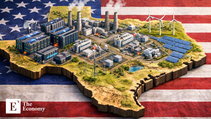
반도체 팹도 텍사스에 자리 잡아
텍사스에 자리 잡기 시작한 반도체 생산 기지들 역시 전력망 부하를 가중하는 요인으로 꼽힌다. 삼성전자는 텍사스 테일러시에 450억 달러(약 66조원) 이상을 투자해 첨단 파운드리 반도체 생산 공장(팹)을 건설 중이다. 앞서 지난해 삼성전자의 미국 법인 삼성 오스틴 반도체(SAS)의 미셸 글레이즈 커뮤니케이션 및 커뮤니티 담당 이사는 2026년 말까지 해당 공장을 가동하는 것이 목표라고 밝힌 바 있다. 테일러 공장은 지난 1월 테일러시로부터 8만8,000제곱피트(약 8,175㎡) 구역에 대한 임시 사용승인서(TCO)를 받고 제한적인 선에서 현장 활동을 시작한 상태다.
일론 머스크 테슬라 최고경영자(CEO)가 주도하는 테라팹 프로젝트의 거점 역시 텍사스다. 테라팹은 텍사스주 오스틴에 건설되고 있는 종합 반도체 기지로, 테슬라 자율주행차 및 휴머노이드 로봇 ‘옵티머스’에 적용될 저전력 추론칩 및 우주 환경에서 구동되는 고성능 AI 칩을 생산할 예정이다. 머스크 CEO가 내건 목표는 테라팹을 통해 연간 1테라와트(TW) 규모의 연산 능력을 확보하는 것이다. 이는 전 세계에서 1년간 생산되는 컴퓨팅 파워(약 20GW)의 50배에 육박하는 수준이다.
이들 반도체 공장은 산업 시설 중에서도 전력 집약도가 높은 축에 속한다. 첨단 파운드리 공장 한 곳은 통상 100~150MW 안팎의 전력을 상시 소비하고, 여러 생산라인이 집적된 대형 캠퍼스의 전력 소모량은 300~500MW를 넘어서기도 한다. 이는 중형 도시 하나가 쓰는 전력에 맞먹는 규모다. 이처럼 대규모 전력 수요가 발생하는 것은 반도체 공정의 특성 때문이다. 반도체 공장에서는 EUV(극자외선) 노광장비와 플라스마·진공 설비, 초정밀 온도·습도 제어가 필요한 클린룸, 화학 공정 설비 등이 24시간 중단 없이 가동된다. 데이터센터, 암호화폐 채굴 시설과 달리 전력망이 불안정해져도 수율 저하 및 손실 문제로 쉽게 가동을 멈출 수 없는 탓이다. 사실상 전력 사용량 조절이 어려운 ‘비탄력 수요’인 셈이다.