[딥파이낸셜] 중국 부동산, 장기 침체의 늪에 빠지나
[딥파이낸셜] 중국 부동산, 장기 침체의 늪에 빠지나

입력
수정
中 부동산 위기 장기 조정 국면 진입
과잉 공급과 수익성 둔화로 일본과 유사한 구조 심화
가계 자산 편중 충격으로 내수 회복이 핵심 변수
본 연구 기사는 유럽 경제 연구소 The Economy의 연구위원(Fellow)들이 작성한 The Economy Review 시리즈 기고문을 한국 시장 상황에 맞춰 재구성한 글입니다. 본 시리즈는 최신 기술-경제-정책 이슈에 대해 연구자의 시각을 담아, 일반 독자들에게도 이해하기 쉽게 전달하는 것을 목표로 합니다. 기사에 담긴 견해는 집필자의 개인적인 의견이며, The Economy 또는 집필자의 소속 기관의 견해와 일치하지 않을 수 있습니다.

중국 부동산 시장 위기가 장기 조정 국면에 들어섰다. 시장에서는 여전히 가격 하락의 저점 형성 시기에 대해 논의가 집중되지만, 핵심 쟁점은 부동산 중심 성장에서 소비 중심 구조로 전환할 수 있느냐다. 중국 경제는 1990년대 일본과 유사한 장기·완만 조정 단계에 접어든 것으로 평가된다. 이러한 흐름은 주요 지표에서도 증명되고 있다.
중·일 부동산 모델의 구조적 유사성
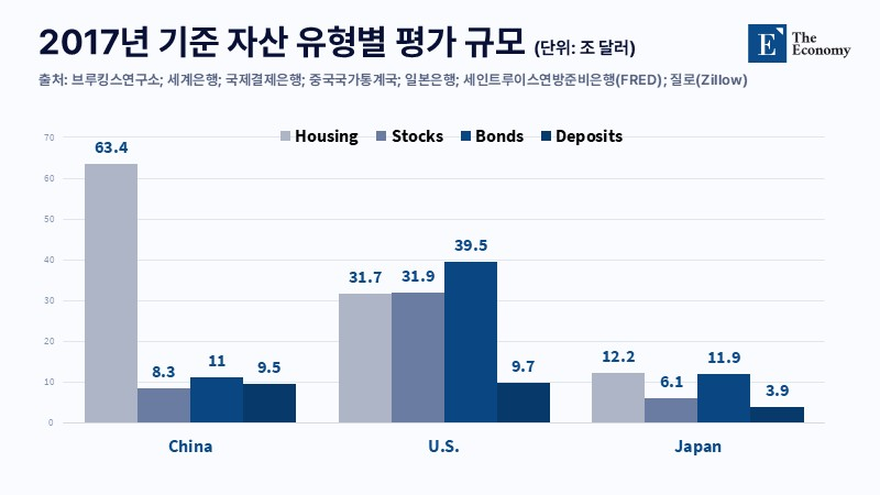
1990년대 일본과 현재 중국의 공통점은 부동산 가격 하락보다, 부동산 투자와 토지 가치 상승에 의존해 온 성장 모델의 한계에서 확인된다. 두 나라 모두 산업 확장과 대규모 투자, 토지 가격 상승 기대를 바탕으로 부동산을 성장 수단으로 활용해 왔다. 그 결과 부동산과 관련 인프라가 전체 수요의 약 3분의 1을 차지하고, 주택이 가계 자산에서 높은 비중을 차지하는 구조가 자리 잡았다.
이 같은 구조는 과잉 건설과 수익성 둔화로 이어졌다. 일본은 붕괴 직전 이미 주택과 인프라 공급이 수요를 넘어선 상태에 놓였고, 중국도 1선 도시를 제외한 지역에서 유사한 흐름이 반복됐다. 중국 지방정부 재정에 기반한 공급 확대가 이어지며 수요를 웃도는 상황이 누적된 결과다. 지난해 부동산 투자 감소와 올해 1분기 두 자릿수 하락세는 투자 대비 수익이 맞지 않는 구조적 한계가 분명해졌음을 보여준다.
통제 가능한 기대 침체와 실물 부담 누적
일각에서는 중국의 강한 국가 통제력과 높은 가계 저축률을 근거로 일본식 장기 침체를 피할 수 있다는 기대가 제기된다. 중국 정부가 개발업체를 선별적으로 지원하며 충격을 분산시키는 방식은 급격한 시장 붕괴를 억제하는 데 일정 부분 기여할 수 있다. 그러나 이러한 대응은 부실을 표면화하지 않은 채 시간을 벌어주는 수준에 그친다. 약화된 가계 신뢰를 회복시키기에는 한계가 뚜렷하다. 부동산 의존 구조에서는 신뢰 약화가 소비 위축으로 이어지며 실물경제 부담을 키운다.
여기에 추가 주택 수요가 남아 있다는 기대도 현실과는 거리가 있다. 현재의 문제는 단순한 수요 부족이 아니라 지역별 수요와 어긋난 공급 구조다. 지방정부 재정과 인센티브가 결합되면서 특정 지역에 공급이 집중됐고, 이는 실제 수요와 맞지 않는 불균형으로 이어졌다. 수익성이 낮아진 이후에도 건설 중심 전략을 유지했던 일본의 경험이 중국에서도 반복되는 모습이다.
가계 자산 편중에 따른 소비 위축 심화
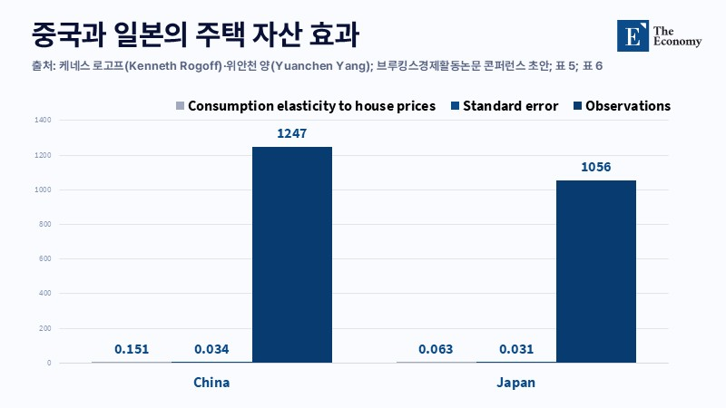
부동산 의존도가 높은 자산 구조는 결국 가계 자산에 직접적인 부담으로 이어진다. 중국 가계 자산의 약 70%가 부동산에 집중된 상황에서 주택 가격 하락은 곧바로 소비 감소로 연결된다. 주택 가격이 20~40% 하락할 경우 소비는 국내총생산(GDP) 대비 2~4% 줄어들 수 있다는 추정도 있다. 올해 1분기 명목 GDP 성장률이 5.0%를 기록했지만, 가계의 재무 여력과 심리는 동시에 약해지는 흐름이다.
이러한 변화는 물가와 대외 지표에서도 드러난다. 소비자물가는 정체 국면을 벗어나지 못하고, 성장의 상당 부분이 대외 수요에 의존하는 구조가 강화됐다. 수출 확대만으로는 부동산발 내수 부진을 보완하기 어렵다는 평가가 힘을 얻는다. 주택이 단순 자산을 넘어 세대 간 안전망 역할을 해온 만큼, 가격 하락에 따른 충격은 자산 감소 폭을 넘어 소비 위축을 확대시키는 요인으로 작용한다.
기로에 선 중국, 일본식 장기 침체 가능성
이러한 흐름은 향후 경로에 대한 우려를 증폭시키고 있다. 일본은 부동산 위기 이전 수준의 주택 가격을 회복하는 데 20년 가까운 시간이 걸렸다. 2024년에 들어서야 토지 가격이 34년 만에 가장 큰 폭으로 상승하며 반등 조짐을 보였을 정도로 조정 과정은 길게 이어졌다. 자산 거품의 후유증이 장기간 경제 전반에 부담을 남긴 셈이다. 중국 역시 이제 조정 초기 단계에 들어선 상황이다. 올해 3월 신규 주택 가격과 상업용 면적 판매 지표는 여전히 시장의 위축된 흐름을 반영한다.
결국 중국의 향방은 내수 기반 재건 속도에 달려 있다. 따라서 토지 매각 의존도를 낮추고 소비 중심 구조로 전환하려면 기득권 저항과 정치적 부담을 감수해야 한다. 미완공 프로젝트 정리와 사회안전망 확충 등 구조 개편이 병행되지 않을 경우 조정 국면은 장기화될 가능성이 크다. 단기적인 GDP 수치나 일부 도시의 가격 반등보다 중요한 중국의 과제는 가계 소비를 회복시킬 기반을 마련하는 데 있다.
본 연구 기사의 원문은 China Real Estate Crisis: Why Japan’s Lost Decades Matter More Than the Official Growth Rate을 참고해 주시기 바랍니다. 본 기사의 저작권은 The Economy에 있습니다.