“하이주얼리 열풍에 혼자 웃는 백화점” K자형 양극화로 나뉜 소비 시장, 전략축도 부유층 중심으로 이동
“하이주얼리 열풍에 혼자 웃는 백화점” K자형 양극화로 나뉜 소비 시장, 전략축도 부유층 중심으로 이동

입력
수정
불황 속 고성장하는 하이주얼리
세금 붙지 않는 상속 수단
희소성 높아 투자 자산으로 인식
중동발 지정학 리스크와 물가 상승 우려 속에서도 주요 백화점들이 뚜렷한 성장세를 보이며 오프라인 소비 회복 흐름을 이어가고 있다. 일부 백화점에서는 하이엔드 주얼리 매출이 두 배 이상 늘며 ‘소비를 넘어 투자로’ 이어지는 흐름이 뚜렷해졌다는 평가다. K자형 소비 형태가 고착화되는 가운데, 중산층 타깃의 매스티지 시장은 쪼그라들고 초고액 자산가 위주로 판이 바뀌고 있다는 분석이 나온다.
3월 백화점 하이주얼리 매출 60% 증가
13일 유통업계에 따르면 롯데·신세계·현대백화점 등 주요 백화점 3사는 지난달 27일부터 시작된 봄 세일 기간 동안 일제히 두 자릿수 매출 증가를 기록했다. 먼저 롯데백화점은 세일 개시 후 첫 주말(3월 27~29일) 기준 전체 매출이 전년 대비 28% 증가했다. 특히 해외 시계·주얼리 매출이 55% 급증하며 전체 실적 상승을 견인했고, 스포츠와 패션 카테고리도 각각 30% 안팎의 성장률을 기록했다.
신세계백화점도 같은 기간 매출이 전년 대비 33.6% 증가하며 3사 중 가장 높은 성장률을 기록했다. 세부적으로는 럭셔리 주얼리가 100.7% 급증했고, 럭셔리 워치도 57.8%의 증가세를 보였다. 아웃도어와 여성·남성 패션도 각각 10~30%대 고르게 성장하며 전반적인 소비 확장세를 뒷받침했다. 현대백화점 역시 같은 기간 매출이 전년 대비 24.8% 늘었다. 시계·주얼리 부문이 56% 증가했고 스포츠와 패션 카테고리도 각각 30% 안팎의 상승률을 보이며 전반적인 소비 회복 흐름에 힘을 보탰다.
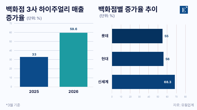
이번 매출 증가의 가장 큰 특징은 하이주얼리 쏠림 현상이다. 롯데·신세계·현대백화점 등 3대 백화점의 3월 하이주얼리 매출 증가율은 작년 같은 기간 대비 평균 59.8%를 기록했다. 신세계백화점의 매출 증가율은 68.3%였고, 현대백화점은 56%, 롯데백화점은 55%였다. 2025년 한 해 동안 3대 백화점에 입점한 하이주얼리 카테고리의 전년 대비 평균 매출 증가율이 33%였다는 점을 고려하면, 올해 3월 증가율은 두드러진다.
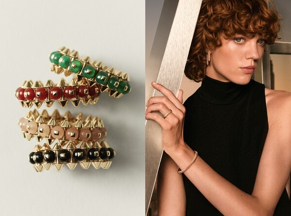
3대 백화점에서 공통적으로 매출이 많이 증대된 하이주얼리 브랜드는 ‘알함브라’ 시리즈로 유명한 반클리프 아펠, ‘왕의 보석상’으로 불리는 까르띠에, 화려한 색감이 특징인 불가리였다. 또 ‘다이아몬드의 왕’ 그라프나 요즘 웨딩 밴드로 인기 있는 부쉐론 등도 매출 상승을 견인했다. 하이주얼리 브랜드의 귀금속 가격은 300만원부터 수억원까지 천차만별이다. 입문용 주얼리라고 불리는 귀금속 가격은 300만~700만원 수준이지만, 고가의 귀금속은 보통 수천만원부터 수억원까지 간다. 통상적으로 목걸이를 하나 사려고 해도 1억원 정도를 지불해야 한다.
투자 목적 수요에 중국인까지 가세
유통업계에서는 하이주얼리 판매 증가의 배경으로, 다주택자의 주택 매도 요인을 지목하고 있다. 집을 매각하고 손에 쥔 돈을 부동산이나 주식 구매로 바로 전환하지 않고 대기시키는 과정에서 그 일부가 하이주얼리로 들어왔다는 것이다. 명품업계 관계자는 "입문용 주얼리보다 5,000만원 이상 고가의 주얼리 판매 건수가 작년 3월 대비 크게 늘었다"며 "목돈 중 일부가 금과 희귀 보석이 포함된 주얼리 매수로 들어온 것으로 해석된다"고 했다.
하이주얼리로 수요가 몰린 또 다른 이유는 ‘희소성’이다. 하이주얼리는 희소성이 높은 고가의 보석과 장인의 기술이 집약된 예술품이라는 시각이 강하다. 사회적 지위를 나타낸다는 점에서 투자나 소장 목적의 구매가 이뤄지고, 품목에 따라서는 시간이 지나도 가치가 떨어지지 않거나 오히려 상승한다. 까르띠에의 경우 평소 연간 1~2회 인상했던 가격을 작년에는 3회 넘게 올렸고 올 1월에도 또 한 차례 인상했다. 1월 27일 가격 인상 전에는 주요 매장마다 사람들이 긴 줄을 서는 진풍경이 벌어지기도 했다. 인기 모델 ‘다무르’의 경우 가격이 크게 올랐는데도 재고가 없어서 당분간 구매조차 어려운 것으로 알려졌다.
하이주얼리를 '손톱만 한 부동산'이라고 부르는 이유도 여기에 있다. 한 유통업계 관계자는 “고소득층이 주얼리를 단순히 사치재가 아니라 투자할 만한 가치가 있는 대상으로 생각하기 시작했다”며 “인플레이션 시대에 자산 가치를 잘 보존할 수 있는 수단으로 여긴다”고 말했다. 또 다른 관계자는 "세금이 붙지 않는 상속 증여의 수단이라는 점까지 감안한 소비가 발생하고 있는 것으로 보인다"고 전했다.
여기에 중국인 관광객의 소비 회복도 실적 개선에 힘을 보탰다. 리서치 및 투자정보 플랫폼 에픽AI에 따르면, 최근 명품 소비 성향이 높은 중국인 관광객이 한일령과 원저 현상에 힘입어 물밀듯이 들어오고 있다. 한일령 이전에는 K컬처에 관심이 많은 중국 젊은 세대가 올리브영, 다이소, 무신사에서 주로 소비했지만, 한일령 이후 명품 쇼핑을 목적으로 일본을 방문하던 중국인들이 한국으로 유입돼 백화점 매출이 큰 폭으로 늘었다는 분석이다.
실제로 롯데백화점은 올해 1분기 전점 외국인 매출이 전년 동기 대비 100% 증가했다. 대표적인 관광 상권으로 꼽히는 서울 명동 본점의 경우 외국인 매출 신장률이 130%를 기록했다. 신세계백화점도 명동 본점 전체 매출이 전년 대비 65% 증가했다. 특히 외국인 매출이 전년 대비 220% 증가하며 실적을 뒷받침했다. 상품군별로는 명품이 120%, 하이주얼리가 56% 성장하는 등 고가 품목 판매 호조가 두드러졌다. 현대백화점 역시 지난달 외국인 매출이 전년 대비 2배가량 증가했으며, 명품(30%)과 하이주얼리(55%) 등 매출 신장률이 높게 나타났다.
K자형 소비 고착화, 백화점 '하이엔드 브랜드'로 돌파구
다만 소비 양극화는 더욱 뚜렷해지고 있는 것으로 분석된다. 고가의 명품과 주얼리는 고성장을 이어가고 있는 반면, 중저가 상품군은 상대적으로 부진한 흐름을 보이고 있기 때문이다. 오랜 기간 부진에 시달려 온 백화점들은 이 같은 K자형 소비 패턴을 고려해 하이엔드 브랜드에 더욱 집중하는 분위기다.
최근 롯데백화점은 반클리프 아펠과 협업해 서울 잠실 롯데월드타워 잔디광장에서 체험형 팝업 ‘스프링 이즈 블루밍’을 진행했다. 1,190㎡(약 360평) 규모의 야외 공간에 설치미술 형태로 구성됐으며, 별도의 사전 예약 없이 누구나 관람할 수 있도록 했다. 이번 전시에는 프랑스 아티스트 샤를로트 가스토의 일러스트 정원이 조성돼 관람객을 맞았다. 파스텔톤 색채로 표현된 정원과 설치 작품들이 공간을 채우고, 꽃 화관 만들기나 정원 꾸미기 등 참여형 프로그램도 함께 선보였다. 현대백화점은 이달 서울 무역센터점 1층에 불가리 팝업 스토어를 열고 대표 제품 ‘세르펜티’ 라인 신제품을 선보일 예정이다.
백화점업계는 명품 브랜드 경쟁력 강화에도 속도를 내고 있다. 롯데백화점은 지난달 인천점에 ‘티파니앤코 플래그십 스토어’를 오픈한 데 이어 이달 인천점에 부쉐론 부티크를 추가로 선보이며 하이엔드 주얼리 라인업을 확대했다. 신세계백화점은 지난해 12월 본점에 까르띠에 부티크를, 같은 시기 광주점에는 불가리 매장을 오픈하며 명품 주얼리 경쟁력을 높이고 있다. 현대백화점도 작년 7월 더현대 서울에 반클리프 아펠을 도입했고 같은 해 12월 판교점에 쇼메 매장을 열며 럭셔리 포트폴리오를 확대하고 있다.
전문가들은 하이주얼리 열풍이 당분간 이어질 것으로 본다. 시장조사업체 인더스트리 리서치에 따르면 하이주얼리 시장 규모는 올해 1,808억 달러(약270조원) 수준에서 연평균 7.8%씩 성장해 2035년에는 3,556억 달러(약530조원)에 이를 전망이다. 하이주얼리 구매자의 약 60%가 초고액 자산가인데, 최근 부의 집중 현상이 강해지면서 이들의 구매력도 커지고 있기 때문이다. 세계적으로 투자 가능 자산이 100만 달러(약 15억원)를 넘는 개인이 2,200만 명을 넘어선 가운데, 특히 아시아 지역의 증가세가 가파르다.