[AI MEMO] AI 규제 경쟁 격화, 美 시장 진입장벽 확대
[AI MEMO] AI 규제 경쟁 격화, 美 시장 진입장벽 확대

입력
수정
美 전 州 AI 입법 확산 부담 현실화
대응 격차 확대, 대기업 중심 재편 가속
기술 격차 축소 속 산업 경쟁력 압박
본 연구 기사는 유럽 경제 연구소 The Economy의 연구위원(Fellow)들이 작성한 The Economy Review 시리즈 기고문을 한국 시장 상황에 맞춰 재구성한 글입니다. 본 시리즈는 최신 기술-경제-정책 이슈에 대해 연구자의 시각을 담아, 일반 독자들에게도 이해하기 쉽게 전달하는 것을 목표로 합니다. 기사에 담긴 견해는 집필자의 개인적인 의견이며, The Economy 또는 집필자의 소속 기관의 견해와 일치하지 않을 수 있습니다.
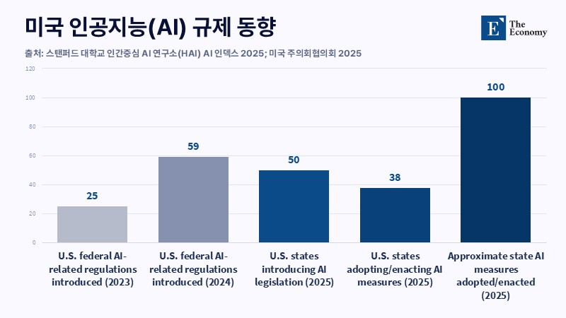
지난해 미국 50개 주 모두가 인공지능(AI) 관련 법안을 발의했고, 이 가운데 38개 주는 약 100건의 규제를 도입했다. 이에 따라 기업은 연방 규제에 더해 빠르게 늘어나는 각 주별 기준까지 함께 검토해야 하는 부담을 안게 됐다. 이처럼 규제가 누적되면서 사업 추진 과정에서 충족해야 할 의무가 늘어나고, 권한이 겹치는 구조 속에서 준수 비용도 함께 커지는 양상이다. AI 규제는 이제 기업과 연구 현장이 직접 감당해야 할 현실적 부담으로 작용하고 있다.
규모의 경제, 규제 대응력 좌우
규제 환경은 빠르게 복잡해지고 있다. 스탠퍼드 2025 AI 인덱스에 따르면 2024년 미국 연방 기관의 AI 규제 발표는 59건으로 전년 대비 거의 두 배로 늘었다. 캘리포니아의 AI 안전법(SB53)은 첨단 AI 개발자에게 안전 프레임워크 공개와 사고 보고 의무를 부과하고, 미준수 시 민사 책임까지 규정한다. 연방과 주 정부 권한이 얽히면서 규제는 다층적으로 쌓이고, 그 부담은 시장 전반으로 확산된다.
그러나 규제의 영향은 기업 규모에 따라 차별적으로 나타난다. 새로운 규정 준수를 위해 필요한 법률 인력, 위험 관리 시스템, 테스트 및 교육 자원은 고정 비용의 성격을 띤다. 자본력이 충분한 대기업은 이를 흡수하며 시장 지위를 강화하는 반면, 자원이 제한된 중소기업과 스타트업에는 진입 장벽으로 작용한다.
이러한 구조는 투자 흐름에서도 확인된다. 2024년 미국 벤처 투자에서 AI 분야 비중은 65%, 약 2,220억 달러(약 326조7,504억원)에 달했다. 하지만 투자 성과는 대형 기업 중심으로 집중되는 경향을 보인다. 규제가 강화될수록 혁신 역량보다 규제 대응 체계를 갖춘 기업이 유리해지는 규모의 경제가 뚜렷해진다. 경제협력개발기구(OECD)도 과도한 행정 부담이 중소기업의 디지털 기술 도입을 제약하는 핵심 요인이라고 지적하며, 규제 준수 비용과 행정 부담이 함께 커지는 위험에 주목할 필요가 있다고 강조한다.
기술 격차 축소와 산업 경쟁력 압박
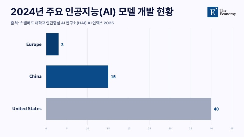
AI 규제 환경은 국가 산업 전략과도 직결된다. 미국은 신규 모델 출시 규모에서 우위를 유지하고 있으나, 후발 주자와의 성능 격차는 빠르게 축소되는 추세다. 올해 3월 기준 스탠퍼드대학교 인간중심 AI 연구소(HAI) 벤치마크에서 미국 최고 모델과 중국 모델 간 성능 차이는 약 2.7% 수준까지 좁혀졌다. 동시에 중국은 논문과 특허, 장비 분야에 대한 투자를 확대하며 기술 추격 속도를 높이고 있다. 이 과정에서 규제 부담이 커질수록 기업의 실행 여력은 제한된다. 그 결과 시장은 성능이 더 높거나 운용 환경이 유연한 해외 기술로 이동하는 경향을 보인다. 이는 자국 AI 산업 기반 약화로 이어지고, 장기적으로는 기술 의존도를 높이는 요인으로 작용한다.
규제 정밀화와 실행 기반 강화
물론 AI가 초래할 수 있는 금융 범죄, 핵심 인프라 장애, 생물안전 위험 등을 고려하면 규제 필요성 자체는 분명하다. 다만 중요한 것은 규제 방식이다. 범위를 넓게 설정한 일반 지침보다 산업별 특성을 반영한 세분화된 기준이 요구된다. 실효성 있는 규제는 명확한 안전지대와 해석 기준을 제시해 기업이 현장에서 적용할 수 있는 운영 기준을 제공해야 한다.
아울러 규제의 실효성은 국가 역량과 결합될 때 확보된다. 규제 기관의 전문성, 테스트 인프라, 공공 조달 체계가 함께 구축되지 않으면 규제는 시장의 예측 가능성만 떨어뜨릴 가능성이 크다. 따라서 중복 규제를 줄이고 감사 체계를 정비하며, 중소기업의 정책 참여를 확대하는 방향으로 규제 정합성을 높여야 한다.
규제 경쟁의 기준 재편
미국 50개 주의 동시 입법은 AI 산업 전반에 규제가 빠르게 누적되고 있음을 보여준다. 이 과정에서 규제 건수를 늘리는 접근이 기술 통제 역량으로 이어진다는 인식도 확산되고 있다. 그러나 이러한 접근은 정책의 초점을 흐리고, 새로운 기술을 실험하고 시장에 진입하려는 주체의 범위를 좁히는 결과로 이어진다. 산업 전반의 활력 둔화 역시 같은 맥락에서 나타난다.
향후 10년의 AI 주도권은 규제 규모가 아니라 운영 방식에서 판가름 날 가능성이 크다. 안전성을 확보하면서도 시장 접근 여건을 유지하고, 장기적 신뢰를 구축할 수 있는 환경을 갖춘 지역이 경쟁에서 우위를 점할 것으로 보인다. 규제가 혁신을 제약하는 장치에 머무르지 않기 위해서는 정책의 초점을 속도보다 방향과 설계의 정교함에 맞출 필요가 있다.
본 연구 기사의 원문은 AI Regulation Is Not Too Uncertain, It Is Too Heavy을 참고해 주시기 바랍니다. 본 기사의 저작권은 The Economy에 있습니다.