장기간 디플레이션에 짓눌려 온 中, 이란 전쟁으로 물가 반등
中 정부의 첨단 산업 육성 정책, 내수 진작 효과는 제한적
국방비 지출 증가 흐름 지속, 내수 회복 정책 '지지부진'

중국 정부가 첨단 제조업 육성에 총력을 기울이고 있다. 장기간 지속된 디플레이션으로 경제 위기가 심화한 가운데, 전략 산업에 대규모 투자를 단행하며 성장 동력 확보에 나선 것이다. 다만 시장에서는 이 같은 정책의 효과가 어디까지나 수출 시장에 국한돼 있으며, 유의미한 낙수 효과를 만들어 내기는 역부족이라는 분석이 지배적이다. 이에 더해 중국의 막대한 국방비 지출 역시 내수 진작을 가로막는 걸림돌로 꼽힌다.

中 물가 흐름 변화 국면

13일 금융권에 따르면, 중국 경제는 지난 수년 동안 강력한 내수 침체 및 디플레이션 압력에 시달려 왔다. 실제 중국 국가통계국(NBS) 자료를 살펴보면 중국 생산자물가지수(PPI)는 2022년 10월부터 지난 2월까지 장장 40개월 동안 마이너스(-)를 기록했다. 중국 소비자물가지수(CPI) 역시 2023년 연간 상승률이 0.2%에 그친 데 이어 지난해까지 사실상 '제로' 수준의 저물가 국면에서 벗어나지 못했다.

상황이 변한 것은 미국·이스라엘과 이란 간 전쟁이 본격화한 올해 3월부터였다. 3월 중국의 CPI는 전년 대비 1%, PPI는 0.5% 오르며 국면 전환 가능성을 시사했다. 지난달에는 이 같은 흐름이 한층 명확해졌다. 지난달 중국 PPI는 전년 대비 2.8% 상승하며 시장 전문가들의 예측(1.53%)을 크게 웃돌았고, CPI 역시 같은 기간 1.2% 뛰며 시장 예상치(0.95%)를 넘어섰다. 중동 분쟁이 글로벌 에너지 가격을 끌어올리면서 물가 오름세가 뚜렷해진 것이다. 국제유가는 이란 전쟁 발발 이후 100달러(약 14만9,000원) 안팎의 높은 수준에서 움직이고 있다.

일각에서는 이러한 물가 반등이 중국 경제에 호재로 작용할 수 있다는 관측이 제기된다. 블룸버그통신은 지난달 "이란 전쟁으로 인한 에너지 가격 상승세가 중국의 디플레이션 부담을 낮춰주고 있다"고 분석한 바 있다. 반면 현재의 물가 변동이 중국 경제에 유의미한 도움이 되지 못할 것이라는 시각도 존재한다. 사우스차이나모닝포스트(SCMP)는 "전쟁에 따른 비용 상승으로 시작된 물가 상승은 수요 증가에 기반한 물가 상승에 비해 기업에 해로울 수 있다"고 경고했다. 지표상의 물가가 개선될 수는 있지만, 실물 경제의 고통은 오히려 더 커질 가능성이 크다는 지적이다.

중국식 '국가 주도 성장'의 허점

이 같은 불확실성 속 중국 정부는 경제 위기를 타파하기 위한 수단으로 첨단 제조업 육성을 낙점했다. 경제협력개발기구(OECD)가 지난 3월 발표한 주요 과학기술 지표(MSTI)에 따르면, 지난 2024년 구매력평가(PPP) 기준 중국의 연구·개발(R&D) 지출은 1조300억 달러(약 1,540조원)로 미국(1조100억 달러)을 처음으로 추월했다. 이는 반도체·인공지능(AI)·전기차·배터리 등 전략 산업을 중심으로 국가 주도 투자가 급증한 결과다.

정부의 산업별 투자 규모를 살펴보면 이러한 기조를 명확히 확인할 수 있다. 먼저 반도체 분야에서는 지난 2024년 3,440억 위안(약 75조원) 규모의 3기 국가집적회로산업투자펀드(빅펀드Ⅲ)가 조성됐다. AI 분야에도 대규모 자금이 투입되는 중이다. SCMP는 뱅크오브아메리카(BofA) 보고서를 인용해 중국의 지난해 AI 설비 투자가 6,000억~7,000억 위안(약 130조~150조원)에 이를 것으로 추산했으며, 이 중 정부 투자만 560억 달러(약 83조원)가량으로 예상된다고 전했다. 전기차 산업에 대한 지원 규모는 한층 크다. 미국 싱크탱크 전략국제문제연구소(CSIS) 분석에 따르면, 중국 정부가 2009~2023년 전기차 산업에 투입한 자금은 최소 2,308억 달러(약 334조7,700억원)로 추정된다.

문제는 중국 정부의 국가 주도 성장 전략이 유의미한 내수 성장으로 이어지지 않았다는 점이다. 현재 중국 내수 시장은 정부 지원하에 불어난 각종 공급을 좀처럼 소화하지 못하고 있으며, 기업들은 남는 물량을 해외 시장에서 처분하는 전략을 채택 중이다. 첨단 산업 역시 내수보다는 수출 부문에서 상대적으로 더 강한 경쟁력을 드러내는 추세다. 이는 정부의 공격적 투자 기조 속에서도 고용 창출과 소비 확대의 순환 구조가 만들어지지 못한 이유다.

정부의 공격적 지원으로 인해 촉발된 '과잉 경쟁' 역시 부작용으로 꼽힌다. 현지 기업들은 정부 보조금과 정책 금융이라는 '안전장치'에 기대 수요 이상의 공급을 쏟아내 왔다. 이로 인해 격화한 시장 경쟁은 가격 인하를 부추겼고, 결국 판매량과 수출 규모가 늘어나는 와중에도 기업 이익은 개선되지 않는 악순환이 시작됐다. 이처럼 기업들의 수익성이 확보되지 않으면 낙수 효과 역시 제한적일 수밖에 없다. 결국 중국 경제는 생산 확대 및 수출 증가에도 불구하고 소비 회복은 여전히 부진한, 이른바 ‘내수 없는 성장’ 구조에 의존 중인 셈이다.

국방비 지출도 내수에 부담

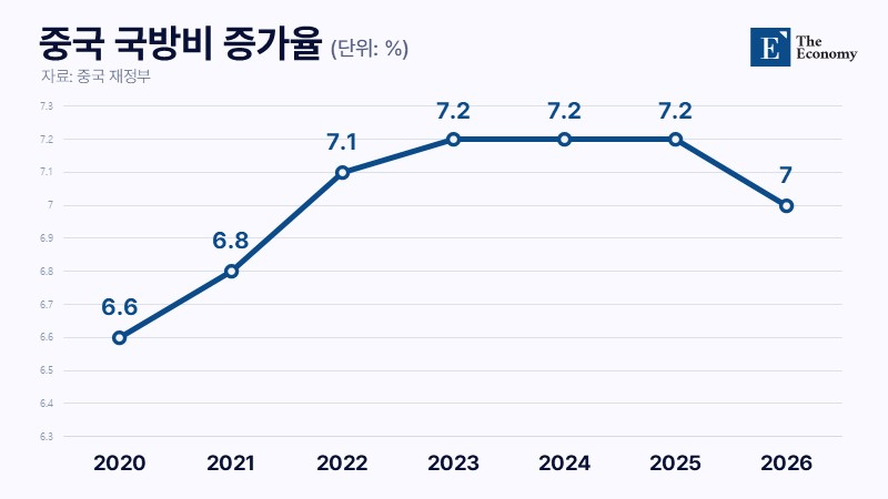
이에 더해 막대한 국방비 지출 역시 내수 침체 흐름을 심화하는 요인으로 거론된다. 중국 국방비 증가율은 시진핑 국가주석 집권 초기인 2012∼2015년 10.1∼12.2%를 기록한 뒤 2016년 7.6%, 2017년 7.0%, 2018년 8.1%, 2019년 7.5% 등 7% 안팎에서 머물러 왔다. 이후 2020년에는 증가 폭이 6.6%로 잠시 둔화했지만, 2020년 10월 ‘건군 100주년’ 목표가 제시된 뒤에는 2021년 6.8%, 2022년 7.1%, 2023∼2025년 7.2% 등 재차 상승세가 이어졌다. 올해 국방 지출 예산은 전년보다 7.0% 늘어난 1조9,096억 위안(약 405조원)으로 책정됐다.

그러나 전문가들은 공식 자료만으로는 중국의 군사 지출 규모를 온전히 파악하기 어렵다고 본다. R&D, 해외 무기 및 장비 구매, 군인 연금 등 예산 외 지출이 집계 대상에 포함되지 않는 데다, 인민무장경찰 및 해안경비대와 같은 준군사조직의 예산 역시 빠져 있기 때문이다. 여기에 중국 특유의 저렴한 인건비 역시 고려해야 할 요인으로 지목된다. 주요 기관들은 이러한 변수를 고려해 각자 상이한 국방비 추정치를 내놓고 있다. 일례로 중국 정부가 발표한 2024년 국방 예산은 2,350억 달러(약 350조원)였지만, 미 상원은 실제 지출을 7,000억 달러(약 1,045조원)로 추산했다. 국제전략연구소는 같은 기간 중국 국방 예산 추정치로 3,300억 달러(약 490조원)를, 스톡홀름국제평화연구소(SIPRI)는 3,175억6,000만 달러(약 475조원)를 제시했다. 미국기업연구소(AEI)는 중국의 실제 국방비가 공식 발표의 3배에 달하며, 2022년 이미 미국의 국방비와 비슷한 수준에 이르렀다고 분석하기도 했다.

문제는 안보 분야 지출이 늘어나며 따라 소비 진작과 내수 회복을 위한 투자 여력이 부족해졌다는 점이다. 실제 중국 정부는 최근 소비 쿠폰·가전 보조금 등 소비 부양책을 내놓고 있지만, 여전히 직접 현금 지급이나 대규모 복지 확대에는 신중한 태도를 유지 중이다. 재정 건전성과 산업 경쟁력 유지에 집중하며 미국식 대규모 소비 부양책에는 선을 긋는 양상이다. 이와 관련해 국제통화기금(IMF)은 최근 보고서에서 중국 경제가 수출·제조업 투자 중심으로 과도하게 기울어져 있으며, 사회 안전망 강화와 재정 지출 구조 변화를 통해 소비 중심 성장으로의 전환을 추구해야 한다고 지적했다.